Rectangles are the most common shape of maps in GIS software, but why stop there?
In GIS software like ArcGIS Pro, it is possible to create map layouts in non-rectangular shapes without too much hassle. But that is not the case in QGIS (yet!), so let’s look at ways to make creative map shapes in QGIS.
In this post, I explain how to download a Sentinel 2 image from the Copernicus Open Access Hub. I want to use this image to make some unique map-layouts.
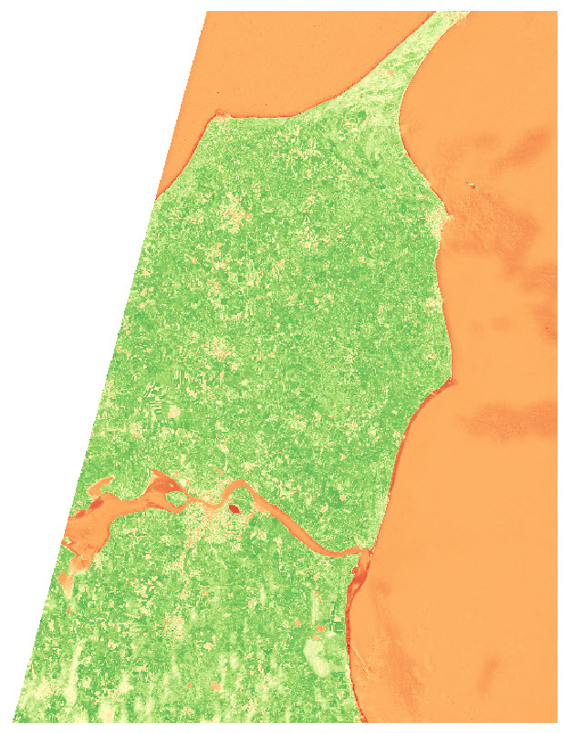
I want to make an NDVI map, so I take the NIR and Red bands from the image (band 8 and 4), add them to QGIS, and use the Raster Calculator to make an NDVI image
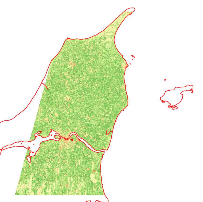
I use the latest country-border polygon from GADM to clip the raster layer
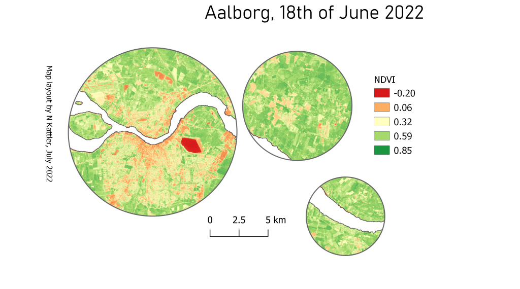
I want to show the NDVI data of the area near the city of Aalborg, in some different shapes.
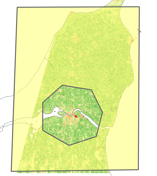
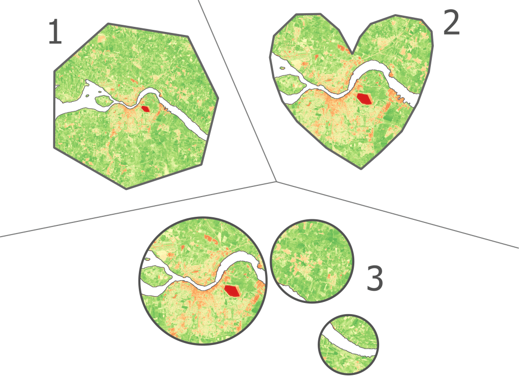
I start by creating two polygon layers, and create a big polygon in one layer and a small polygon (near Aalborg) in the second layer . The small polygon is the one that will define the layout, so get creative!
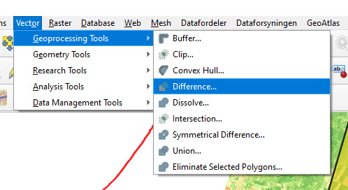
I use the Difference tool in QGIS to cut out the shape of the small polygon in the large polygon.
The outcome looks something like this:
Depending on your creative skills, you can make some cool shapes. You can also import a pre-made polygon and use that instead.
Here are the 3 versions I ended up with:
You can also add some of the classical map elements
Personally I don’t find the Copernicus Open Access Hub very intuitive to use, so I wanted to provide an example of how I download data from the website.
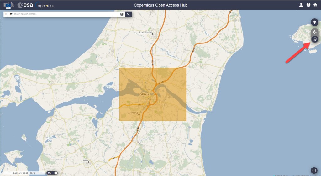
For this example I want to download a single Sentinel 2 (A or B) image from the northern part of Jutland in Denmark. I want it to be cloud free and it should be as recent as possible.
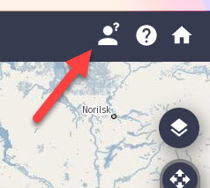
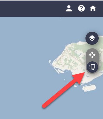
2. Click on “Switch to Navigation Mode” in order to select the area that you are interested in
3. Select the area
4. Click on the filter-button left of the search bar, and make the following selections:
Select Sort by : Sensing date
Select the time period you are interested in (choose Sensing period)
Select the Sentinel satellite mission you want data from Tip: If e.g. you just want any image from Sentinel 2, you don’t have to select anything in the Satellite platform dropdown, just leave it empty.
Select cloud cover % if that is relevant. For Sentinel 2, I usually set the cloud cover very low, e.g. “[0 to 10]”.
5. Click on the search symbol in the top, and you should see a list of available images from your area. If you don’t see any images, try to change the cloud cover or expand the selected time period.
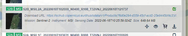
6. Select the image that suits your needs and download it. The download might take a while. The most recent image I downloaded took ~3 min to download and the size was ~0.6GB.
How a filter could look like
The image I ended up selecting
Once the download is finished, the next challenge is to find the raster files in the labyrinth of subfolders. I found mine here:
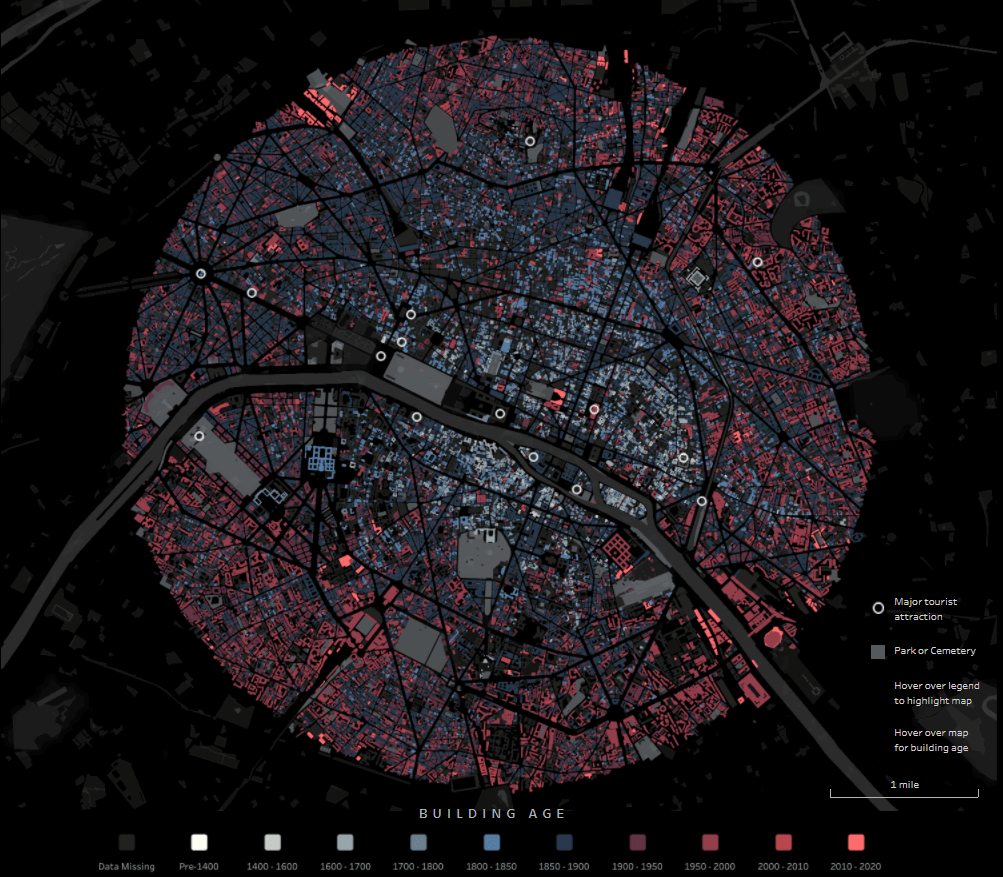
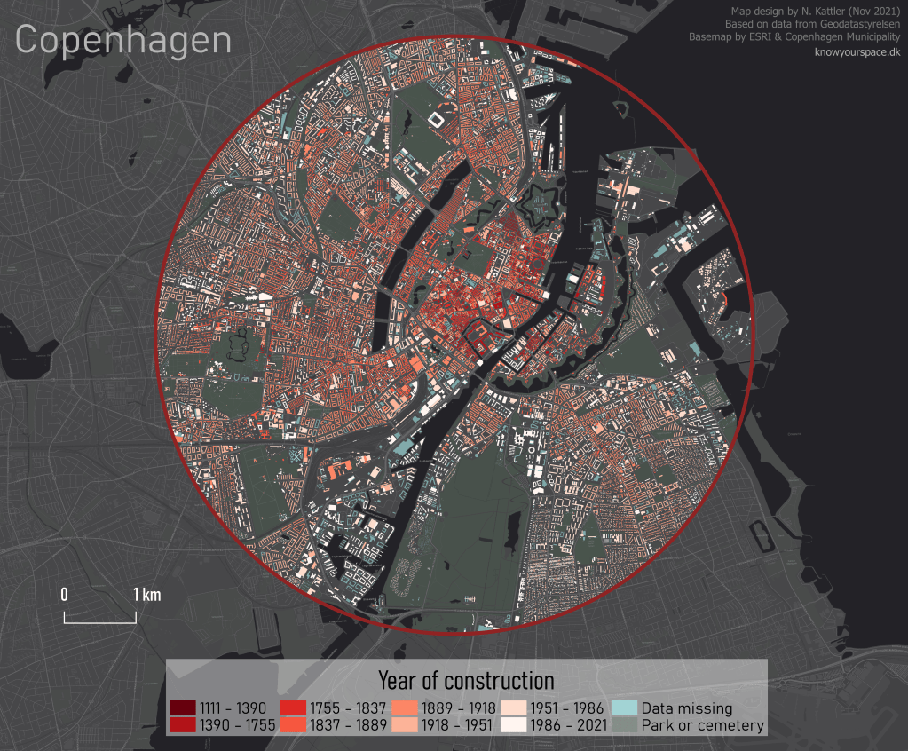
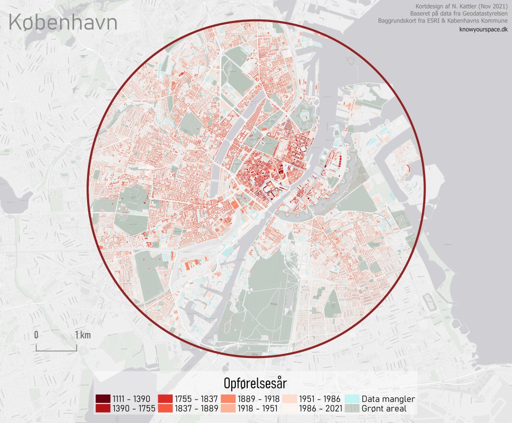
Through the exellent newsletter quantum of sollazzo by Giuseppe Sollazzo (@puntofisso) I learned of the beautiful map of Paris by Naresh Suglani (@SuglaniNaresh), where Suglani have visualised the year of construction in a lovely blue-to-red colour gradient. It is a stunning visualisation, and I immediately wanted to try to make a similar version myself.
Here you can see Suglani’s original:
“Paris | Building Ages” by Naresh Suglani. September 2021.
In order to recreate this map I needed to get my hands on 1) the shapes of buildings in Copenhagen and 2) the year of construction.
The shape of buildings
Dataforsyningen is part of the Danish Agency for Data Supply and Efficiency, and they offer a range of datasets. One of them is the dataset INSPIRE – Bygninger. This dataset follows the INSPIRE directive by the European Union, which promotes the standardisation of the infrastructure for geographical data in Europe. The file contains polygons of the shape of buildings, which is what I needed. The file format is GML, which you can read about here.
This is a rather big file, because it is not possible to filter which part of Denmark you are interested in.
The age of the buildings
Unfortunately, the GML file does not contain a “date of construction” attribute, so I had to find that elsewhere.
From my current workplace, I know of a dataset called “BBR”, which stands for Bygnings- og Boligregistret (Building- and Housing Registry). This dataset contains information about housing plots, buildings, facilities etc. in a point format. I had a strong suspicion that BBR includes information about the year of construction, so I downloaded the dataset from Dataforsyningen, just like the buildings-dataset. This dataset is called INSPIRE – BBR bygninger og boliger, and comes in the geopackage file format (.gpkg).
Once again, we get a rather large file:
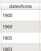
I open the file and — we are in luck! The point-file contains an attribute called “dateofcons” aka date of construction.
However, one thing stood out: Several buildings had the date of construction as the year 1000. Now I am no history major, but that seemed like a bit of a stretch. So I asked around, and it turns out that the BBR-dataset use the value 1000 as their “unknown” category. Not the most ideal choice in my opinion, but that’s how it is. Therefore I had to filter out the 1000-values in the dateofcons column for my visualisation.
Clipping the data
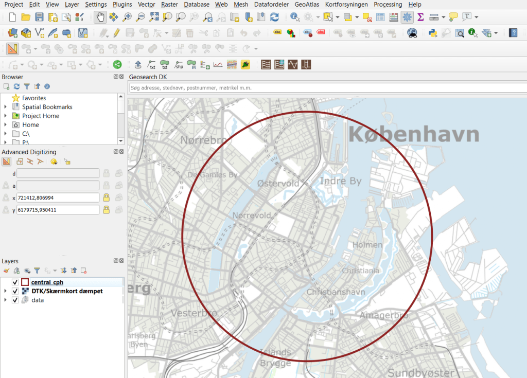
To follow the design of Suglani, I focused on central Copenhagen. I created a circular polygon encompassing most of the old town of central Copenhagen to use to clip the two datasets.
Then I was ready to clip the data to fit my circle:
And here are the results:
Building polygons to the left, BBR points on the right.
Next I needed to join the two datasets somehow, so that each building could have an attribute with its year of construction. For this I needed to do a join attributes by location.
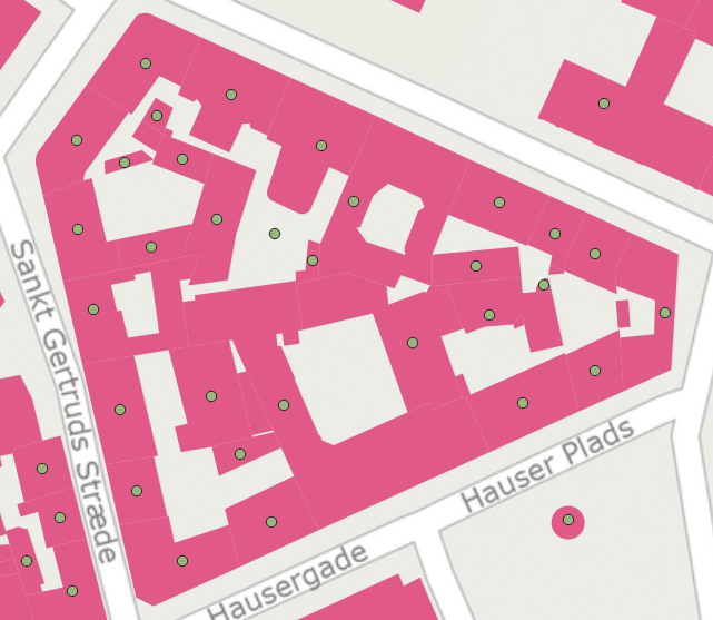
By doing this kind of join I assumed that both datasets are near-perfect, i.e. that all buildings are registered at a high level of detail, and that the position of the BBR-points will not fall out of the building polygons. That is a large assumption to make, and there will probably be some errors. Let’s have a closer look at how well the two datasets match:
I would say this is an excellent fit, although there is at least one BBR-point which seems to be floating in the air, with no building-polygon nearby.
I ran the join tool, waited a few minutes, and voilá!
QGIS is not as easy to work with regarding spatial statistics as its commercial counterpart ArcGIS. However, QGIS does have some plugins that can do some great statistical analysis. One example is the Attribute Based Clustering plugin, created by the QGIS-contributor ekazakov.
The logo of the plugin
The plugin creates clusters based on the attributes of a vector layer, not the spatial distribution of the data. The clusters are calculated using either a hierarchical or a k-means algorithm. If you are using the hierarchical clustering, you can define the weight of each attribute that you want to include in the cluster analysis. The higher the weight, the stronger the effect, or impact, the attribute will have on how the clusters are created. You can read more about the plugin on ekazakov’s own website which includes a tutorial of the plugin.
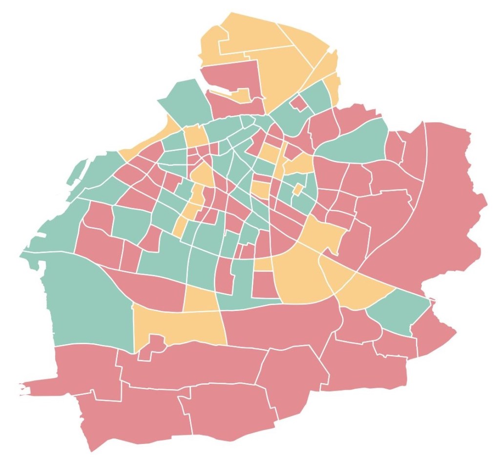
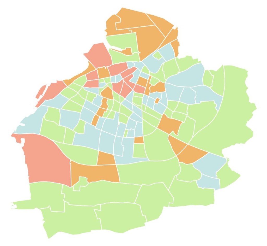
I recorded a video for a GIS course where I give an example on how you can use the plugin, and what the result looks like, using data from Malmö, a city in southern Sweden.
Sorry for the low video quality! I’ll try to explore the settings of the recording software next time.
The data was from Malmö Stad and can be downloaded here as an Excel file. The three attributes that I used were:
Amount of people with a longer education (“Eftergymnasial“) in 2019
Amount of people with a foreign background (“Utländsk bakgrund“) in 2019. NB: This number includes people born in the country, but where both parents are foreigners.
Percentage of the population who are employed (“Förvärvsarbetande“) in 2018
Below you can see the difference between having 3 and 4 clusters, using the same settings otherwise: